Image Classification without Labelled Data using OpenAI Clip - Part 1

A series on OpenAI Clip

Deep learning has dramatically changed the way we write software and build new technologies in the past 10 years. From the GPT family of models capable of generating highly convincing texts, to diffusion models that provide controllable image and video generation at unprecedented quality, the list goes on and on of new applications of deep learning to problems that were previously intractable.

However, despite recent advances, many common problems such as object detection and segmentation, image classification, building models for driverless cars etc require high quality labelled data. For example to build a model that recognizes different categories of cars, you have to collect hundreds or thousands of pictures of each type of car, label it with human annotators and then train a fully supervised model to recognize the types of new cars. This is the common practice today and it comes with two challenges.

1. Collecting and labelling large amounts of data is expensive and in some problem domains, it is not feasible.

2. Models trained in this fashion cannot generalize to new categories without collecting new data and retraining. For example, if you train a model with two car types, “Volvo” and “Toyota”, and you supply a new image of a “BMW”, it will classify it as either Volvo or Toyota without ability to recognize if it is a completely new type of car.

The first problem is often alleviated with transfer learning from large datasets such as ImageNet, however, models trained on ImageNet transfer poorly to data domains that are not related to the images contained in ImageNet. Hence, the representations learned from ImageNet classification generalize poorly to many real world problems.

To solve both problems, Alec Radford et al published the paper, “Learning Transferable Visual Models From Natural Language Supervision (arxiv.org)” in 2021.

CLIP, an abbreviation of Contrastive Language Image Pretraining, learns from the vast unlabeled pairs of image and associated texts such as captions from the internet by mapping the images and texts into the same embedding space. After training, CLIP can be used to build new image classifiers. You simply specify the names or text descriptions of new object categories to be classified and clip can classify any new images into any of the categories you have specified (this is called zero-shot classification) or even recognize that the new image doesn’t fall into any of the categories you specified. All without training, the only training is the pretraining that has been done on images and text pairs from the internet. Also, due to the fact that clip was trained on internet scale data, it can generalize to new types of images including sketches, drawings, synthetic data, and so forth that would prove very challenging to fully supervised ImageNet models.

In addition to image classification, CLIP can be used for semantic search and the image and text representations learned by CLIP can be used as feature extractors in other types of models as seen in diffusion models.

Fig. 1. ZeroShot Clip vs Imagenet Resnet101 on classification of banana pictures from different image types

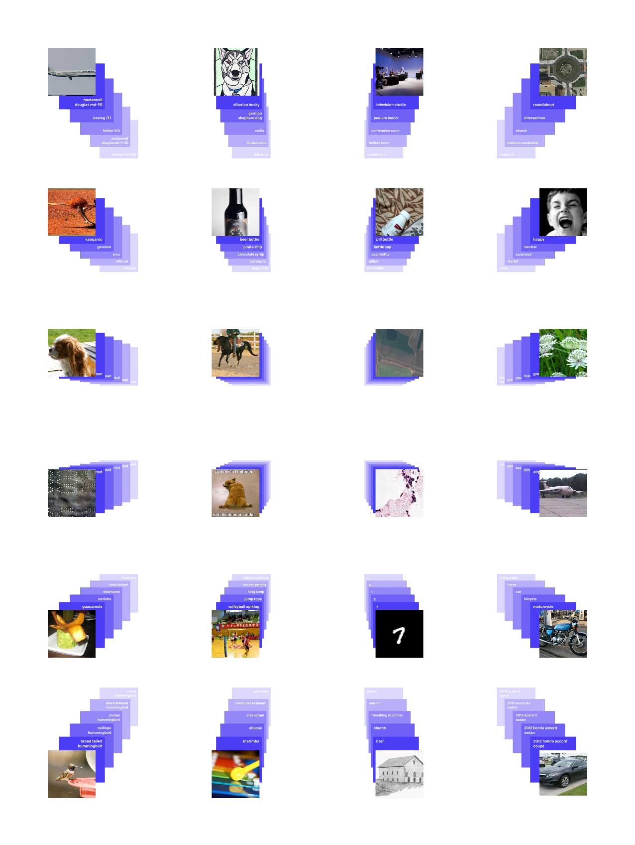
In fig 1 above, we have different pictures of bananas, the first row contains normal pictures of bananas as can be found in the ImageNet dataset, the next rows contain different variants of banana pictures including sketches. As humans, we can recognize bananas from either a picture or a sketch, we want AI models to be capable of doing the same. To this end, a resnet101 model trained on ImageNet was tested against these different image types and we can see how the accuracy drops as the image types change. Zero-shot CLIP was tested against this as well and it significantly outperforms the resnet model trained on ImageNet by a wide margin. This is without training CLIP to specifically classify bananas, it relies on the facts that there are lots of banana pictures on the internet in different representations including sketches.

Building a new Classifier in a few Lines of Code

I have talked a lot about CLIP, now let’s see it in action by building a new image classifier on categories of our liking without collecting any data or training any new model. Simply follow the steps below.

• Install Pytorch and TorchVision using

pip3 install torch torchvision torchaudio

Note, if you have a fast GPU and you want to install pytorch with GPU support, follow instructions at https://pytorch.org

• Install some dependencies

pip3 install ftfy regex tqdm

• Install OpenAI Clip

!pip install git+https://github.com/openai/CLIP.git

Now that we have all the dependencies installed, let’s create a classifier with the following set of categories.

“A car on the road”, “A car in the desert”, “A boat on water”

The above are interesting categories that require an understanding of the content of the image and the context.

Next, below we shall create the function to load the CLIP model, the category names and define a predict function.

import torch
import clip
from PIL import Image

# Run model on cpu or GPU
device = "cuda" if torch.cuda.is_available() else "cpu"

# Load clip model
model, preprocess = clip.load("ViT-B/32", device=device)

# Define category descriptions
categories = ["A car on the road", "A car in the desert", "A boat on water"]
text = clip.tokenize(categories).to(device)

# Define function to predict new images
def predict(image_path):

    # preprocess the image
    image = preprocess(Image.open(image_path)).unsqueeze(0).to(device)

    with torch.no_grad():

        # find cosine similarity of the image to the categories
        logits_per_image, logits_per_text = model(image, text)
    
    # retrieve index of category with highest cosine similarity
    class_index = logits_per_image.argmax().item()

    # retrieve score of best class
    logit_score = logits_per_image.max().item()

    class_description = categories[class_index]

    print(f"Category: {class_description}, Score: {logit_score}")  

Now, lets test this function with a few images.

Test with Image of Car on the Road

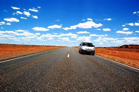
predict("image1.jpg")

Category: A car on the road, Score: 27.453125

Test with Image of Car in the Desert

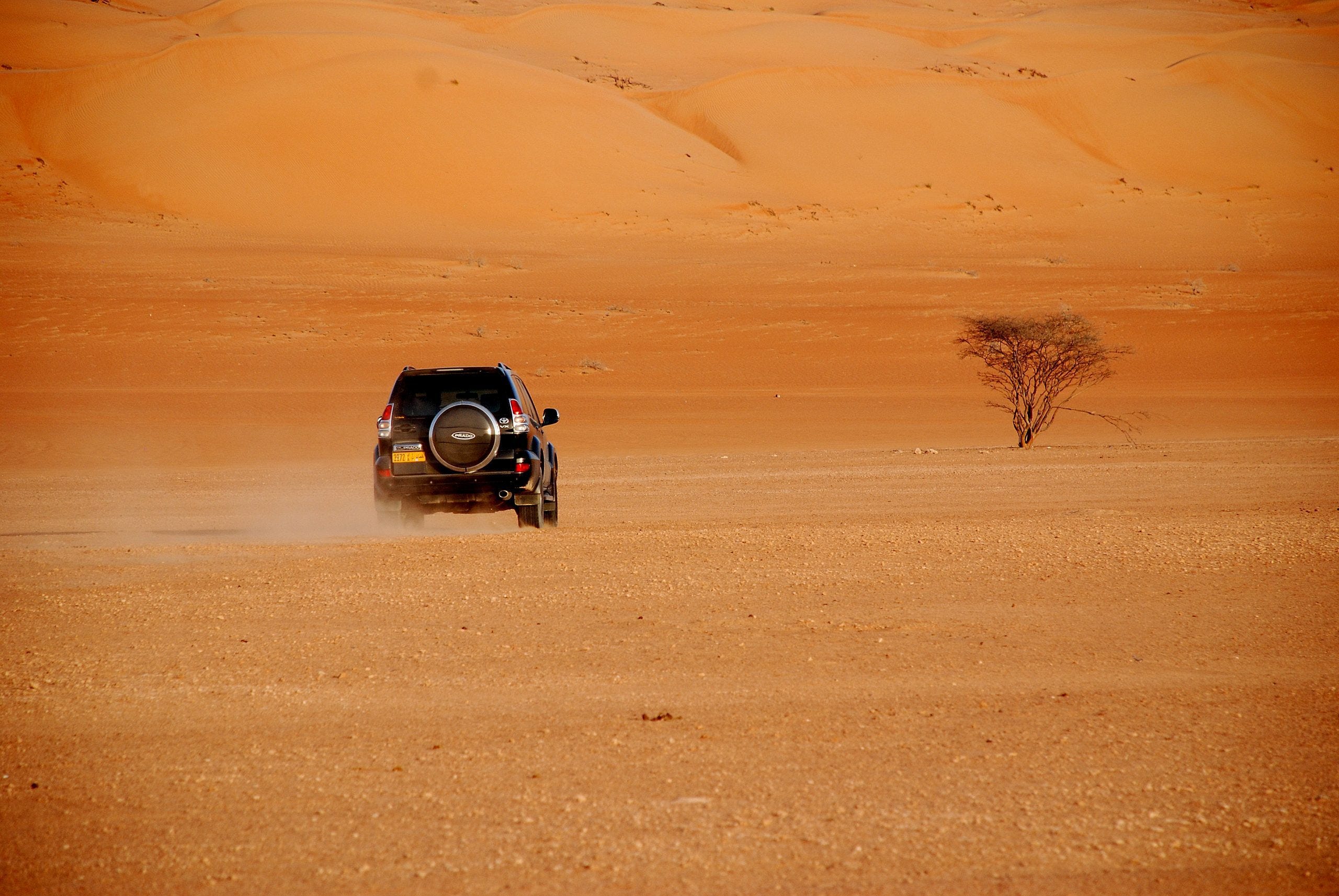
predict("image2.jpg")

Category: A car in the desert, Score: 30.609375

Test with Image of Boat on Water

predict("image3.jpg")

Category: A boat on water, Score: 24.125

Test with Image of Lion Roaring

For this test, we want to see how the model does on a picture of an image outside of the categories we have defined.

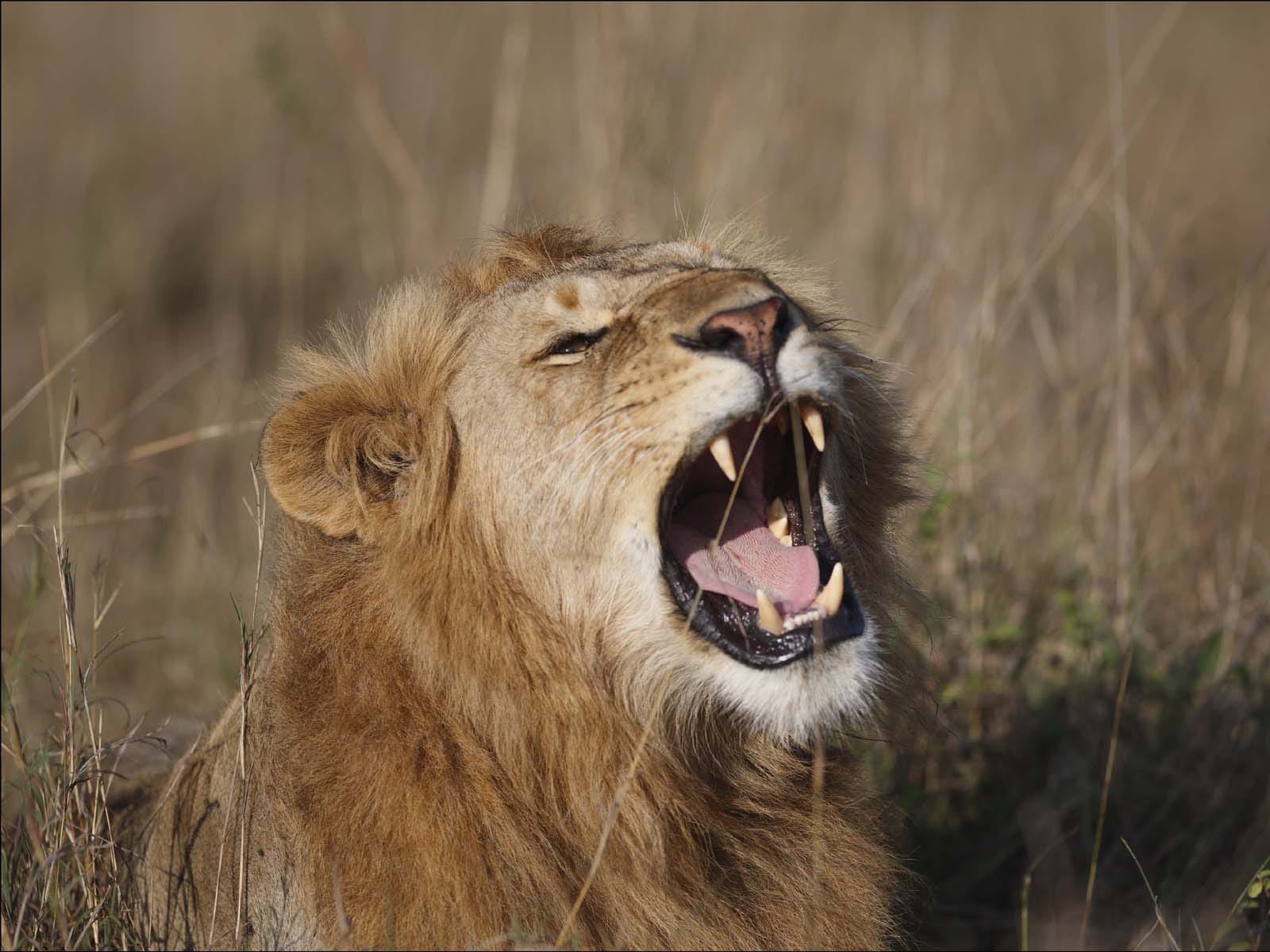
predict("image4.jpg")

Category: A car on the road, Score: 16.90625

Here is an interesting result, the nearest match to the lion image is “ A car on the road” but notice that the score is quite low, in this case 16.9 while for the other images above, the score is at least 24. The logit score would range between 0 - 100.

This allows us for example to filter out any images which gets a score of less than a threshold. For instance, we could say that any image that has a score lower than 22 would be unknown.

Now, let’s see what happens when we tell our model to actually support classifying images of lions, this is as simple as adding an extra text to the list of categories, see code below.

import torch
import clip
from PIL import Image

# Run model on cpu or GPU
device = "cuda" if torch.cuda.is_available() else "cpu"

# Load clip model
model, preprocess = clip.load("ViT-B/32", device=device)

# Define category descriptions
categories = ["A car on the road", "A car in the desert", "A boat on water", "A lion in the jungle"]
text = clip.tokenize(categories).to(device)

# Define function to predict new images
def predict(image_path):

    # preprocess the image
    image = preprocess(Image.open(image_path)).unsqueeze(0).to(device)

    with torch.no_grad():
        
        # find cosine similarity of the image to the categories
        logits_per_image, logits_per_text = model(image, text)
    
    # retrieve index of category with highest cosine similarity
    class_index = logits_per_image.argmax().item()

    # retrieve score of best class
    logit_score = logits_per_image.max().item()

    class_description = categories[class_index]

    print(f"Category: {class_description}, Score: {logit_score}")

Above, we have added the text “A lion in the jungle” to the list of categories. Let’s see how this changes our classification of the lion image.

predict("image4.jpg")

Category: A lion in the jungle, Score: 26.390625

Great! It classified the lion image correctly with a high score of 26.

Note how we just added support for a new class in our model without needing to collect any data or do any retraining, that is the power of CLIP.

HOW CLIP WORKS

At the core of clip is the concept of contrastive training. Unlike supervised training setups, in contrastive learning, data from two or more input modalities such as images, text, audio etc are encoded into a similar latent space by minimizing the distance between correct pairs and maximizing the distance between incorrect pairings.

As shown in the diagram above, to train clip, we take an image of a bird and a text description as downloaded somewhere from the internet. The image is encoded into an embedding space by an Image Encoder network, this would be a VisionTransformer or a resnet model, the text is encoded into an embedding space using a transformer model. Now, we want to align the two embedding that came from the image text pair.

This is where the magic happens. In batch of image-text pairs, let’s say a batch of 10 items (10 images and 10 associated texts), the total number of possible pairings of 10 images and texts is 10**2 = 100 pairs. Out of this 100, we know only 10 pairs are correct, therefore there are 100 - 10 = 90 incorrect pairs.

In summary, in batch of N image texts, there are N correct pairs and N**2 - N incorrect pairings. CLIP is trained to minimize the cosine distance between the N correct pairings and maximize the cosine distance between the N**2 - N incorrect pairings.

The intuition here is that visual concepts in images or texts should map to a similar embedding. This can then be utilized for zero shot image classification, search or transfer learning.

Training Clip

The ability of CLIP to model such a large variety of visual concepts and generalize across different types of images and texts is largely due to the fact that it was trained on 400 million image text pairs from the World Wide Web. While labelling such a large amount of data would have been nearly impossible, the pairs of image texts were derived from associated texts like captions, alt-text, etc that can be easily scrapped from the web without labelling. Some of this would surely be noisy, but with large enough data, the model is able to work well. This enables not just standard classification, but also enables CLIP to do things like recognize actions (people laughing or fighting), perform OCR even though it wasn’t trained to do OCR, geo-localization etc. This follows a trend of large language models developing new abilities they were not trained to do due to the large amount of data used to trend them.

Besides the scale of data, the other key component that makes CLIP so good is transformers.

The transformer architecture, Vaswani et al 2017 ([1706.03762] Attention Is All You Need (arxiv.org)), has enabled hyper scaling of deep learning models. Compared to prior architectures such as Convolutional Neural Networks and Recurrent Neural Networks, the abilities and accuracy of transformers scale really well with increase in data and compute. ([2010.14701] Scaling Laws for Autoregressive Generative Modeling (arxiv.org)).

Therefore, the text encoder of CLIP used the standard transformer and the image encoder used the VisionTransformer ([2010.11929] An Image is Worth 16x16 Words: Transformers for Image Recognition at Scale (arxiv.org))

More details on how CLIP was trained and how to train CLIP from scratch on your own would be explained later in this series.

Summary

CLIP, like all large language models, is pretty amazing. Using a combination of big data and transformers, we can learn a single model capable of performing image classification without retraining, while generalizing across different types of images.

In the next part of this tutorial, we shall explain how to implement image search, similar to the way the Photos app on iOS allows your type in a query and return all matching images. We shall build a simple demonstration using the power of OpenAI CLIP to search a library of images using texts such as “pictures of cats”.

Github Repo

Code and images used in this tutorial is in my github repo here, johnolafenwa/OpenAIClipTutorial

Subscribe

If you enjoyed reading this and would love to read more, please subscribe to this publication here.

About the Author

I am a scientist at the Microsoft Research Lab, Cambridge, United Kingdom, where I have built and shipped deep learning solutions to millions of people. As a machine learning researcher with a strong background in software engineering, my interests and expertise cuts across multiple computer science disciplines including generative models, large language models, convolutional neural networks, DevOps, and cloud native computing.

You can reach to me on johnolafenwa@gmail.com or on twitter @johnolafenwa